This project focuses on the development of a computer vision system for boat classification. The main objective is to detect the presence of boats in images and determine whether they are docked or navigating. We present the decisions made regarding data transformations, architecture, hyperparameters, and results obtained in this work.
1. Methodology
1.1. Image Preprocessing: Data Augmentation
The data transformations were performed taking into account the domain characteristics, including horizontal flips, rotations of no more than 5 degrees, random adjustments of brightness, contrast, and saturation, and Gaussian blur. We highlight RandomCutout, a class created to randomly cut a rectangle in any part of the image, not exceeding a given cut ratio. All these transformations were applied randomly using RandomApply.
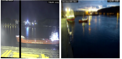
Figure 1: Example of transformed images.
Since a model pretrained on ImageNet images is used, normalization and resizing techniques based on that dataset's parameters were adopted.
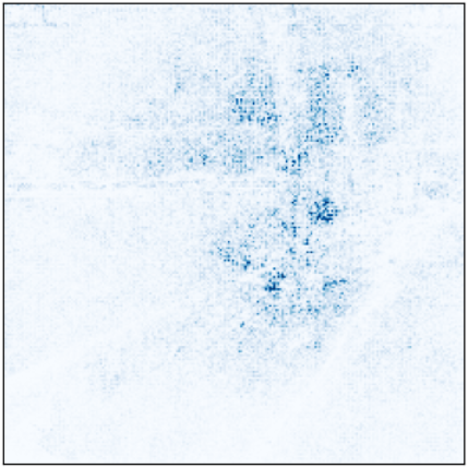
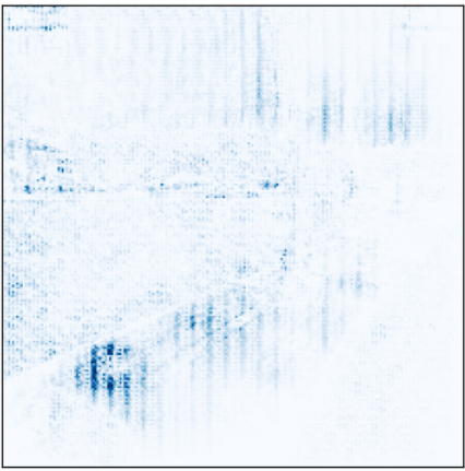
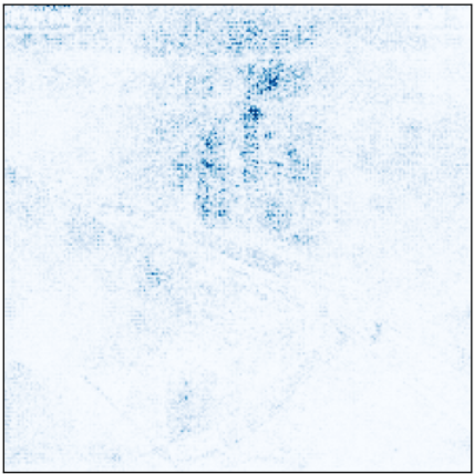
The decision to resize images directly (considering potential quality loss) and not add padding was because, in model training, it focused on the added black borders rather than the image. We can observe this with the help of Captum. In Figure 2, we show which regions the pretrained model without data augmentation paid more attention to when predicting a test image (the model is the one with the lowest loss in the validation set, across all k folds).
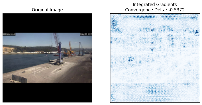
Figure 2: Attention in model regions (with padding).
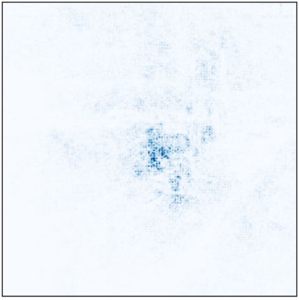
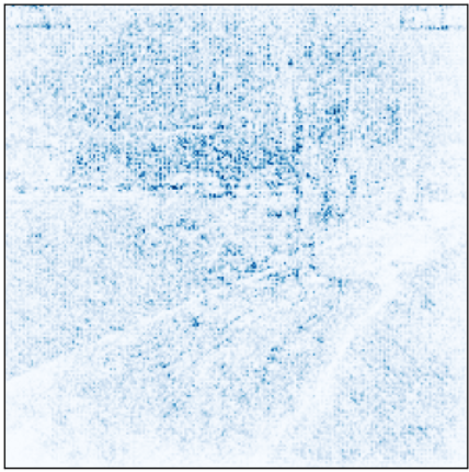
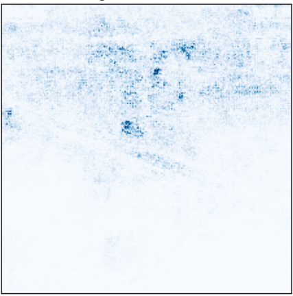
And we see how for the same model (Figure 3), changing only the way data is transformed, it focuses on more specific parts of the image. This approach improves metrics on the test set (Table 1).
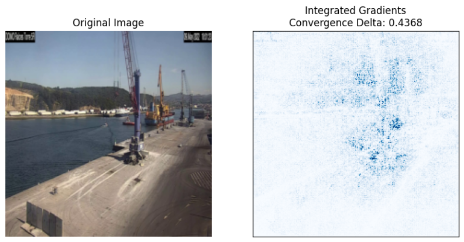
Figure 3: Attention in model regions (without padding).
| Metric | Model with Padding | Model without Padding |
|---|---|---|
| Test Accuracy | 0.93 | 0.95 |
| Test Recall | 0.9232 | 0.9375 |
| Test F1 | 0.9287 | 0.9461 |
| Test Precision | 0.9367 | 0.9605 |
| Test AUC | 0.9738 | 0.9905 |
Table 1: Comparison of metrics between model with and without padding.
1.2. Neural Network Architecture
The architecture used is MobileNet, a not very complex architecture. Modifying the last layer to perform binary classification.
1.3. Training and Validation Strategies
Stratified k-fold with k=5 was used to ensure folds maintained a balanced class distribution. Additionally, a sampler was implemented during training to balance classes in each batch. Earlystopping technique was used, and the best model of each fold was stored according to the loss metric.
The selection of these hyperparameters depended fundamentally on the model weights initialization, as in models with random weights, convergence was much slower.
| Metric | Pretrained | Random weights |
|---|---|---|
| Epochs | 12 | 25 |
| Patience | 3 | 11 |
| Learning rate | 0.001 | 0.01 |
| Optimizer | ADAM | ADAM |
| Criteria | Cross entropy | Cross entropy |
Table 2: Selected hyperparameters
2. Experiments and Results
2.1. Boat/No-boat Classification Model
Below, we present the graphs of metric evolution in the validation set for the four models (with/without data augmentation and with/without random weights).
I. Pretrained model without data augmentation (preT_wF):
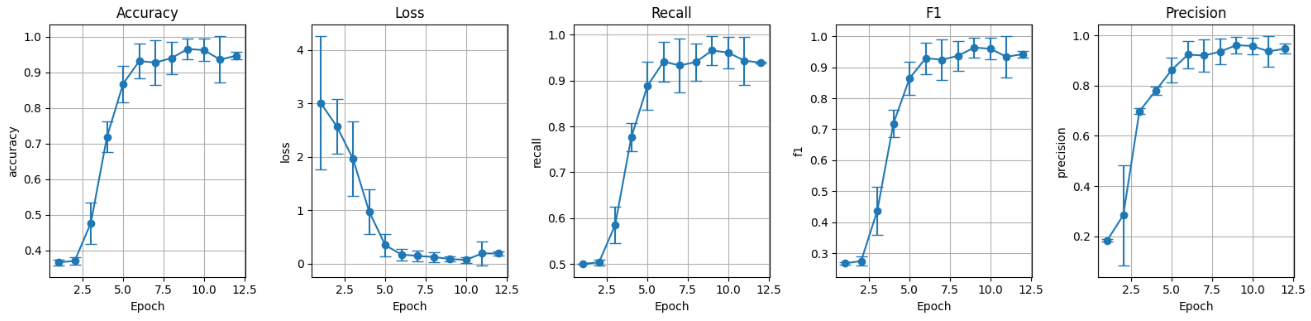
Figure 5: Validation set metrics pretrained without data augmentation.
II. Pretrained model with data augmentation (preT_wT):
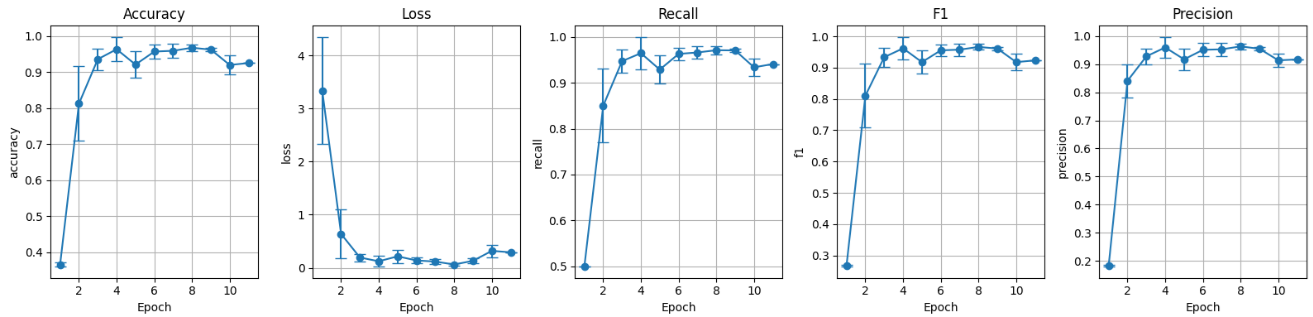
Figure 6: Validation set metrics pretrained with data augmentation.
III. Random weights without data augmentation (preF_wF):
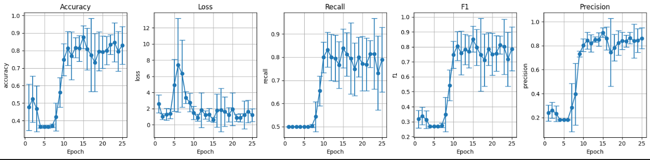
Figure 7: Validation set metrics random weights without data augmentation.
IV. Random weights with data augmentation (preF_wT):

Figure 8: Validation set metrics random weights with data augmentation.
We show the metrics (Table 3) and ROC curves (Figures 9, 10, 11, and 12) on the test set of the k models obtained for each initialization (as indicated before, in each fold we stored the one with the lowest loss in the validation set).
| Model | Accuracy µ | Accuracy σ | Recall µ | Recall σ | F1 µ | F1 σ | Precision µ | Precision σ | AUC µ | AUC σ |
|---|---|---|---|---|---|---|---|---|---|---|
| preT_wF | 0.93 | 0.02 | 0.9083 | 0.0250 | 0.9197 | 0.0227 | 0.9446 | 0.0136 | 0.9688 | 0.0116 |
| preT_wT | 0.92 | 0.02 | 0.9092 | 0.0279 | 0.9139 | 0.0225 | 0.9260 | 0.0142 | 0.9805 | 0.0061 |
| preF_wF | 0.85 | 0.03 | 0.8232 | 0.0332 | 0.8354 | 0.0338 | 0.8793 | 0.0311 | 0.8992 | 0.0410 |
| preF_wT | 0.84 | 0.03 | 0.8149 | 0.0322 | 0.8269 | 0.0330 | 0.8752 | 0.0280 | 0.9195 | 0.0190 |
Table 3: Mean and standard deviation of best model metrics per fold in test.
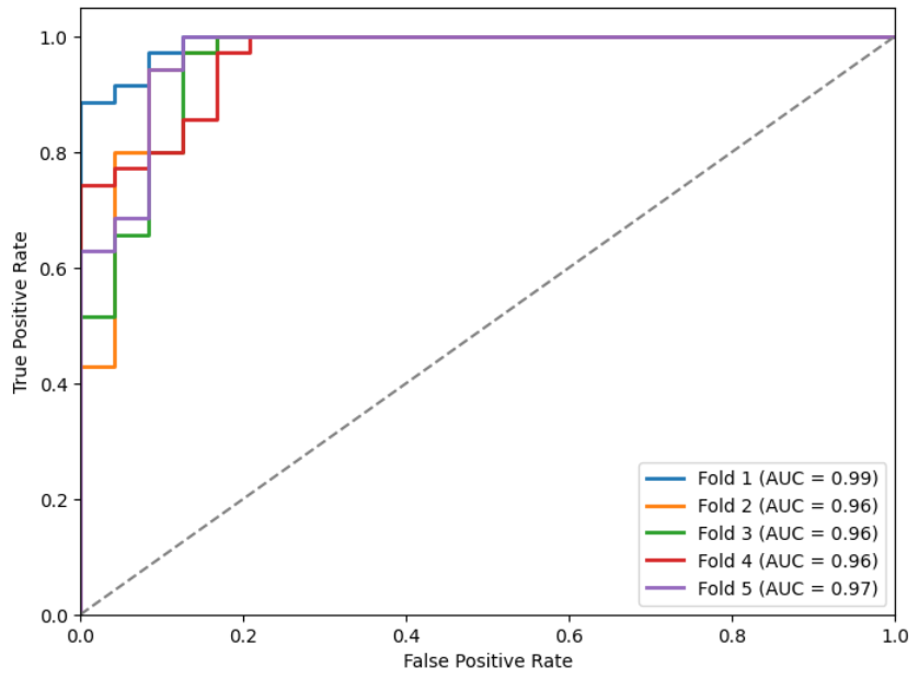
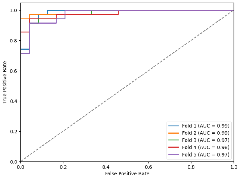
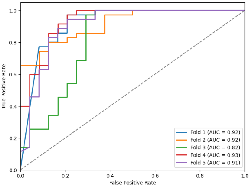
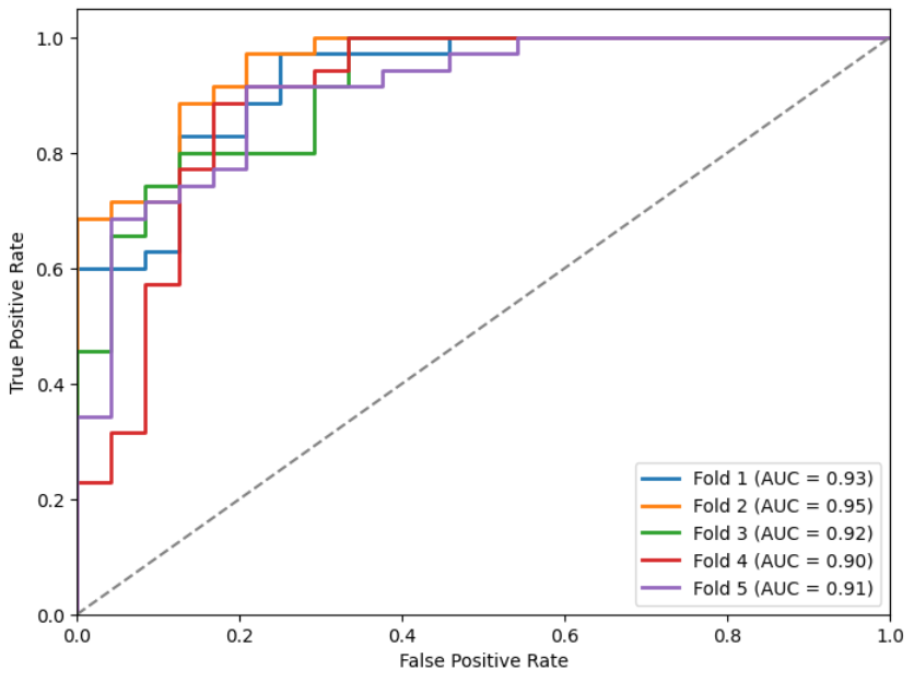
Figures 9, 10, 11, and 12: ROC curves for the different models.
Finally, we show the metrics of the best model for each initialization (understanding by best, the one with the lowest loss in the test set, not in validation).
| Model | Accuracy | Recall | F1 | Precision | AUC |
|---|---|---|---|---|---|
| preT_wF | 0.9492 | 0.9375 | 0.9461 | 0.9605 | 0.9905 |
| preT_wT | 0.9322 | 0.9232 | 0.9287 | 0.9367 | 0.9893 |
| preF_wF | 0.8983 | 0.8750 | 0.8891 | 0.9268 | 0.9333 |
| preF_wT | 0.8644 | 0.8464 | 0.8550 | 0.8731 | 0.9262 |
Table 4: Model metrics
It seems very interesting to see how the 4 models are able to classify Figure 3 shown previously correctly, but paying attention to different parts of the image.
Figures 13, 14, 15, and 16: Attention of models preT_wF, preT_wT, preF_wF, and preF_wT.
2.2. Docked/Not-docked Boat Classification Model
For this model, we use the previously trained model that obtained the best loss. And we train it following the same process, but instead of 4 different models, we will use the one already trained with data augmentation.
Training metrics on the validation set:
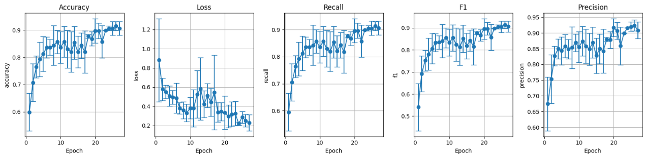
Figure 17: Validation set metrics pretrained with data augmentation.
Metrics and ROC curves on the test set of the best models per fold:
| Model | Accuracy µ | Accuracy σ | Recall µ | Recall σ | F1 µ | F1 σ | Precision µ | Precision σ | AUC µ | AUC σ |
|---|---|---|---|---|---|---|---|---|---|---|
| preT_wT | 0.87 | 0.05 | 0.8687 | 0.0484 | 0.8679 | 0.0496 | 0.8835 | 0.0342 | 0.9427 | 0.0218 |
Table 5: Mean and standard deviation of best model metrics per fold in test.
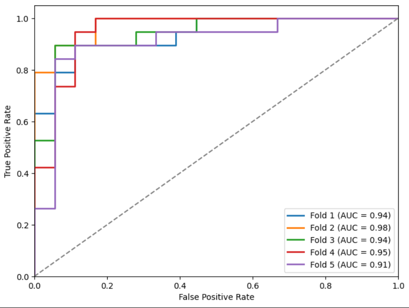
Figure 18: ROC preT_wT.
Metrics of the best model on the test set:
| Model | Accuracy | Recall | F1 | Precision | AUC |
|---|---|---|---|---|---|
| preT_wT | 0.9189 | 0.9196 | 0.9189 | 0.9196 | 0.9766 |
Table 6: Statistics of the preT_wT model
Finally, it is interesting to see again how the attention of the new model changes compared to the previous pretrained one:

Figures 19, 20, and 21: Original image, attention model preT_wF (boats), and attention model preT_wT (docked boats).